Introduction

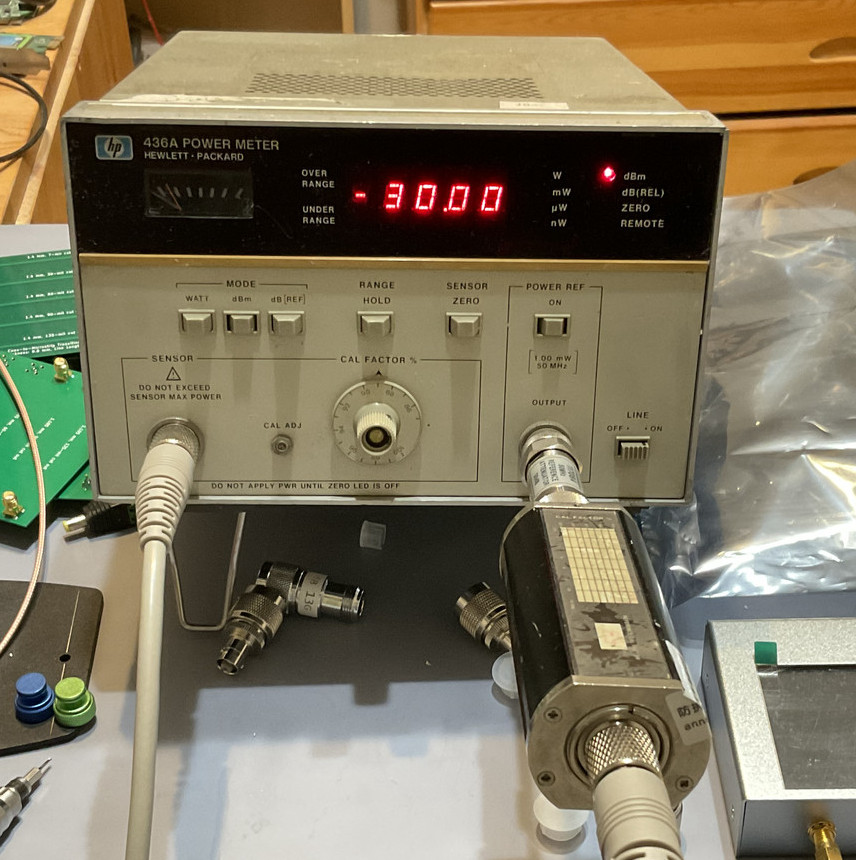
Recently, I’ve purchased a vintage Hewlett-Packard 436A RF power meter and a HP 8484A power sensor for testing a circuit I’m building. Since the measurement I’m trying to do is delicate, on the order of 0.1 dB, I need to estimate my measurement accurary and to understand the sources of uncertainties.

In this article, the main sources of uncertainties in RF and microwave power measurements are explained.

This article belongs to the Tech Note section of this blog, which is a section of notes for my personal understanding and future reference about a technical subject. It’s not necessarily within the interests of all readers, and the quality may not be high enough. But hopefully still useful to some.

In particular, the rigorous and systematic method of calculating uncertainties according to the Guide to the Expression of Uncertainty in Measurement (GUM) is intentionally omitted due to its mathematical complexity.

Mismatch Uncertainty

An imperfect impedance matching and the infeasibility to measure the complex reflection coefficients create the biggest source of RF measurement uncertainties.

Sensor Mismatch Loss

Let’s consider an ideal RF signal generator, which is connected to an ideal transmission line. An imperfect RF power sensor is attached at its end. Since the RF power sensor is imperfect, its complex input impedance $Z_{\text{sensor}}$ is not exactly matched to the system impedance $Z_0=50\mathrm{\Omega }$, this gives rise to a non-zero complex reflection coefficient ${\mathrm{\Gamma }}_{\text{sensor}}$.

When the radio wave travels down the line and hits the sensor, instantly, a portion of the incident power is reflected back to the source.

$$P_{\text{reflected}}=P_{\text{incident}}\cdot {|\mathrm{\Gamma }|}^2$$

The reduction of transmitted power to the sensor due to reflection is known as the mismatch loss, which is given by:

$$\begin{array}{rl}{\text{Mismatch Loss}}_{\text{dB}}& =10\cdot {\log }_{10}(\frac{P_{\text{incident}}-P_{\text{reflected}}}{P_{\text{incident}}})\\ \text{ Let }{P}_{\text{incident}}=1\\ & =10\cdot {\log }_{10}(1-P_{\text{reflected}})\\ & =10\cdot {\log }_{10}(1-{|\mathrm{\Gamma }|}^2)\end{array}$$

where $|\mathrm{\Gamma }|$ (sometimes $\rho$) is the magnitude of the sensor’s complex reflection coefficient. This can be calculated or measured from its input impedance:

$$\mathrm{\Gamma }=\frac{Z-Z_{\text{0}}}{Z+Z_{\text{0}}}$$

Here, knowing the complex form of $Z$ or $\mathrm{\Gamma }$ is unnecessary, since only its magnitude $|\mathrm{\Gamma }|$ is used. Thus, it can be determined from a Standing Wave Ratio or return loss measurement using inexpensive instruments.

For example, let’s assume the sensor’s input impedance is almost matched to the system impedance, say $Z_{\text{sensor}}=(51-20j)\mathrm{\Omega }$, so $|\mathrm{\Gamma }|=|0.047-0.188j|=0.2$ (14 dB return loss, SWR is 1.5). This is not a perfect match, but is not too bad - it indicates only 2% of the incident power is reflected (20% in voltage), giving a mismatch loss of $10\cdot {\log }_{10}(1-{0.19}^2)=0.16\text{ dB}$.

If the signal generator is ideal, that would be the end of it - when the reflected power hits the signal generator, it’s dissipated inside the generator and no longer plays a role. Just add 0.16 dB to the measured power, and this measurement error is fully corrected. In fact, this error is absorbed into the Calibration Factor of the power sensor, thus it’s already compensated for.

Measurement Mismatch Loss

Unfortunately, in the real world, the signal generator is not ideal. Due to physical imperfections of the RF connector and circuit components - just like the sensor, it’s unable to fully maintain the ideal system impedance. With a complex output impendace $Z_{\text{source}}\ne Z_0$, a non-zero complex reflection coefficient ${\mathrm{\Gamma }}_{\text{source}}$ arises.

When the reflected power from the sensor hits the signal generator, a portion of that reflected power is re-reflected again towards the sensor, and when it hits the sensor, a portion of power is subsequently reflected back to the source again, ad infinitum.

Worse, the reflected power can add constructively or destructively to the incident power depending on its phase shift. Thus, the measurement mismatch loss is not just the sum of two individual mismatch losses, but is instead given by:

$${\text{Mismatch Loss}}_{\text{dB}}=10\cdot {\log }_{10}(\frac{{|1-{\mathrm{\Gamma }}_{\text{source}}{\mathrm{\Gamma }}_{\text{sensor}}|}^2}{1-{|{\mathrm{\Gamma }}_{\text{sensor}}|}^2})$$

Quite unexpectedly, we can show that the imperfect power sensor can sometimes receive more power than what would be received by a perfectly matched sensor, unlike what is suggested by the name mismatch loss. This happens when we’re especially unlucky and the reflected power has the correct phase to add constructively to the incident power. In a similar way, when the phase is aligned destructively, the received power in the system can be more than the sensor’s mismatch loss, and may create a significant error.

For example, a perfectly matched sensor has $\mathrm{\Gamma }=0$ by definition, thus it’s trivial to show ${\log }_{10}(1/1)=0$, the mismatch loss is 0 dB, or none. But now suppose the generator’s complex reflection coefficient is $\mathrm{\Gamma }=0.029+0.196j$, and the sensor in the previous example has $\mathrm{\Gamma }=0.047-0.188j$, the calculated mismatch loss is -0.17 dB, or a gain of 0.17 dB above the power absorbed by the ideal load.

This is easier to understand in the language of circuit theory, in this case, the source, $Z=(49+20j)\mathrm{\Omega }$, and the sensor, $Z_{\text{sensor}}=(51-19j)\mathrm{\Omega }$ just happen to form a conjugate match - one has an inductive impedance, another has a capacitive impedance, the imaginary parts cancel out, giving the maximum power transfer.

Uncertainty

If the complex reflection coefficients $\mathrm{\Gamma }$ of both the source and the sensor are known, this error can be fully corrected using the equation above. This is known as a Gamma Correction.

Unfortunately, this is often infeasible due to many practical difficulties. For one, measure the sensor is easy, but ${\mathrm{\Gamma }}_{\text{source}}$ can be complex to measure (no pun intended). It can be a signal generator with an output level dynamically adjusted by an Automatic Level Control circuit, or an amplifier driven to point of saturation - in both cases, the system is highly non-linear and requires special measurement techniques. It also depends on the exact measurement setup - any change of cables or adapters will change the phase shift, foring a painstaking remeasurement. Thus, we often only know $|\mathrm{\Gamma }|$, but not $\mathrm{\Gamma }$.

Without the knowledge of phase, the best we can do is correcting the $1-{|\mathrm{\Gamma }|}^2$ term first (applying the sensor’s calibration factor), then calculate the upper and lower limits of the uncertainty due to phase shift. This can be done by setting the term ${|1-{\mathrm{\Gamma }}_{\text{source}}{\mathrm{\Gamma }}_{\text{sensor}}|}^2$ to two extreme values:

$$\begin{array}{rl}{\text{Lower Bound}}_{\text{dB}}& =10\cdot {\log }_{10}{(1-|{\mathrm{\Gamma }}_{\text{source}}||{\mathrm{\Gamma }}_{\text{sensor}}|)}^2\\ & =20\cdot {\log }_{10}(1-|{\mathrm{\Gamma }}_{\text{source}}||{\mathrm{\Gamma }}_{\text{sensor}}|)\\ {\text{Upper Bound}}_{\text{dB}}& =20\cdot {\log }_{10}(1+|{\mathrm{\Gamma }}_{\text{source}}||{\mathrm{\Gamma }}_{\text{sensor}}|)\end{array}$$

This is known as the Mismatch Uncertainty.

For example, a signal generator and a sensor with $\mathrm{\Gamma }=0.2$ (SWR = 1.5) have an uncertainty of $[-0.35\text{ dB},+0.34\text{ dB}]$.

Nevertheless, in real experiments, it’s extremely unlikely that a 180-degree phase shift is encountered in every single data point, and one can argue this uncertainty is overtly pessimistic. Indeed, sophisticated statistical models are available for reducing this uncertainty solely based on an assumption of $\mathrm{\Gamma }$’s probability distribution. Nevertheless, using these models require the knowledge of statistics and metrology, thus the worst-case uncertainty is often used in practical daily works.

It’s also worth pointing out that because phase shift is a function of frequency (the complex impedance and reflection coefficient just keep rotating around the Smith chart). If the frequency span is large enough, both values will be encountered at some point in an experiment. When doing measurements in a seriously mismatched setup using a spectrum analyzer with a tracking generator, this creates a “ripple” effect in the frequency response plots.

When the device-under-test has a significant impedance mismatch, measurement quality is visibly degraded. A good way to reduce mismatch uncertainty in this scenario is adding an attentuator in front of the device.

Calibration Uncertainty

An imperfect sensor calibration is also a major source of measurement uncertainties.

Calibration Factor

When an RF power sensor is made, the factory makes an initial calibration to see how much the power readings deviate from an ideal sensor. Subsequently, this difference in percentage is printed onto the sensor as a Calibration Factor (CF) table.

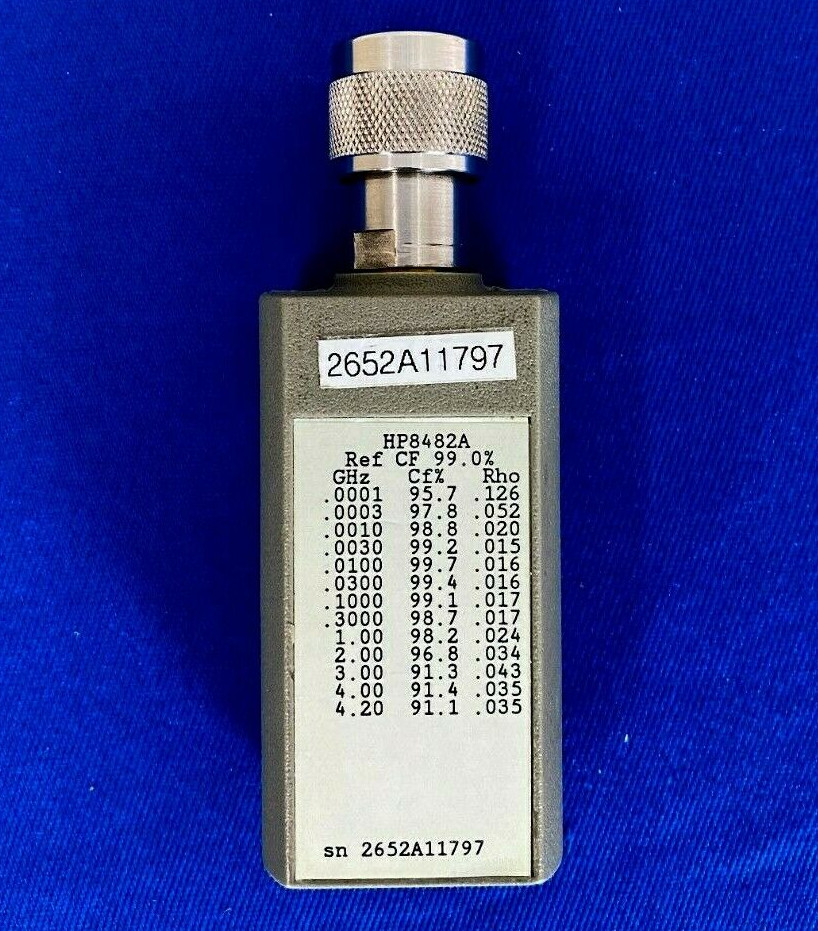
Image by eBay vendor advancedtestequipment, fair use.

To help users to calculate a more realistic mismatch uncertainty rather than taking the datasheet’s maximum limits, the sensor’s reflection coefficients are often also measured simultaneously. Sometimes even the phase is available in a seperate paper report provided along with the sensor.

This calibration corrects two errors. First, the mismatch loss of the sensor itself. As explained previously, because of impedance mismatch, a small portion of the source’s available power never enters the sensor. Next, the effective efficiency (${\eta }_e$) of the sensor. This represents the senser’s ability to produce a reading proportional to input power. These two errors are related to the Calibration Factor by this simple relationship:

$$\text{CF}={\eta }_e\cdot \underset{\text{Mismatch Loss}}{\underbrace{(1-{|\mathrm{\Gamma }|}^2)}}$$

Using the sensor in the picture as an example, at 1 GHz, the mismatch loss is $10\cdot {\log }_{10}(1-{0.024}^2)=0.002\text{ dB}$, thus, at a few gigahertz, the imperfection of the actual sensing element ${\eta }_e$ is almost solely responsible for the measurement errors, not the impedance mismatch.

Effective Efficiency

Just because the power enters the sensor doesn’t imply it’s actually metered by the sensing element, a small amount of power can get lost due to the lossy conductor, circuit components, or radiation. Moreover, due to the imperfections of the sensing element, its DC output is not exactly proportional to the incoming power, especially across the frequency spectrum.

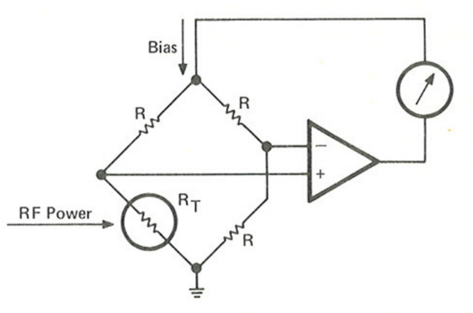
It’s called efficiency, because the original thermistor sensors operate by the principle of RF/DC substitution - the incoming RF power is dissipated in a resistor bridge circuit, while the sensor also dissipate its own DC power in the resistor bridge. The system reaches equilibrium when the temperature increase due to RF heating is the same as what would be caused by DC heating. Thus, ${\eta }_e={\text{P}}_{\text{DC}}/{\text{P}}_{\text{RF}}$ These thermistor power sensors have slow respose and not sensitive to low power, thus they have become antiquated in the industry, and are only used in calibration labs due to their high accuracy.

For the thermocouple and diode sensors, common in modern times, however, the imperfect effective efficiency is mostly due to non-ideal characteristics of the sensing elements, for example, due to a diode’s deviation from the square law across frequencies. Thus, effective efficiency is defined as a ratio between its DC reading and the RF input power, and is not a true efficiency.

Uncertainty

In the ideal world, applying the Calibration Factor according to the RF signal frequency you’re measuring should completely correct all errors of a particular power sensor.

Unfortunately, a calibration lab is not magic, it encounters all the same uncertainties described in this article, albeit it controls them better. Thus, Calibration Factors themselves have associated uncertainties, and are documented in the sensor datasheet or your calibration report.

For example, this is the specification of the HP 8482A power sensor.

A Sum of Uncertainties is the worst-case uncertainty by adding all sources of uncertainties together, while a Probable Uncertainty is the statistically-more-likely Root Sum Square (RSS) of all uncertainties. See Appendix 1.

Some RF power sensors, especially thermistor sensors but also some modern sensors, are physically capable of achieving higher accuracy than the factory calibration uncertainty. In fact, off-the-shelf commercial sensors are frequently calibrated by national standard labs and used as inter-laboratory comparison standards.

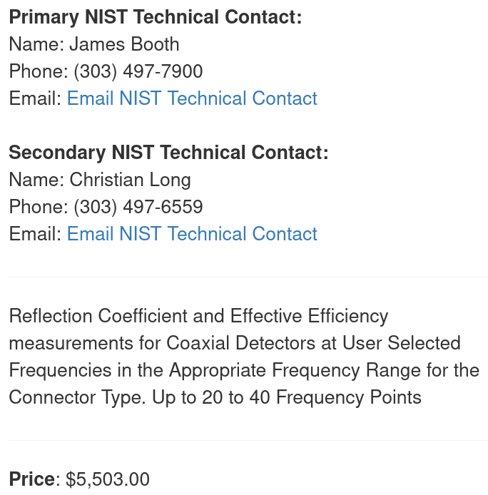
For example, the HP 478A thermistor sensor has a factory calibration uncertainty of 1.4%, but at NIST, 0.3% to 0.7% is achievable.

Thus, you can improve a sensor’s calibration uncertainty by redoing the calibration at the best lab you can afford. For example, in the United States, the National Institute of Standard and Technology will never let you down… For a price around $5000. If you do choose this route, don’t forget to handle the sensor carefully in the future (e.g. before making any connection from your sensor to other devices, you should use a $3000 connector gauge - basically a specialized micrometer - to measure the connector’s pin depth to avoid physical damages by low-quality, out-of-spec connectors), and recalibrating it again frequently… Wear and tear from daily uses can change sensor characteristics.

Sensor Non-linearity

At high power levels, thermocouple sensors can have a slightly non-linear response.

Some of the latest power sensors are calibrated at different power levels and use a multi-dimensional calibration factor table, and is applied under digital control, thus eliminating this error. But this is a problem for older sensors, which are only calibrated at a single level and depends on sensor’s linearity to provide accurary results.

The HP 8481A, 8482A, and 8483A have a worst-case uncertainty of [-4%, +2%] (-0.18 dB, +0.09 dB) when operating between 10 dBm and 20 dBm, and negligible otherwise. Diode sensors are not affected. Always remember to read the manuals.

Reference Uncertainty

In an old-school thermistor power sensor that operates by principle of RF/DC substitution, the heat generated by the incoming RF power is constantly compared with the sensor’s DC power. This is called a closed-loop measurement, the sensor, once calibrated, does not need further adjustments. Component drifts are automatically compensated, because the drift has the same effect to the DC power as well.

But for the thermocouple and diode sensors, common in modern times, it’s an open-loop measurement. The measured power is whatever the sensing element reads, there is no inherent compensation for component drifts. Thus, RF power meters have a built-in 50 MHz reference signal generator. It uses Automatic Level Control to ensure the output power remains at 0 dBm (1 milliwatt), and is periodically recalibrated. Each time before the sensor is used, one first connects it to the power reference and fine-tunes the meter’s offset control to get a 0 dBm reading, thus ensuring accurary.

However, calibrations of the power reference itself are never perfect, thus introduces a small uncertainty to all measurements - typically 1%. For example, the HP 436A power meter’s reference is factory calibrated to 0.7% within the NIST reference, one-year uncertainty is 0.9% RSS and 1.2% worst case (0.052 dB).

When the sensor is connected to the reference for initial adjustment, the mismatch loss uncertainty also applies, but it’s in the range of 0.01 dB and can be neglected (50 MHz is a low frequency, and easy to maintain perfect impedance matching).

Instrumentation Uncertainty

After the sensor finshed its job of generating a DC voltage proportional to RF power, the final uncertainty is introduced by the imperfection of DC voltage measurement by the power meter - which is a seperate apparatus, connected to sensor via a cable.

This is the usually the smallest component of measurement uncertainties and is usually neglected. For the HP 436A power meter, it’s only 0.5% (0.02 dB).

There are also some miscellaneous uncertainties, consult your manuals for more details. On the HP 436A, there are:

1. Zero set uncertainty - only 1 count on most ranges, effectively a rounding error. But at the lowest range it can be 0.5% Full Scale (not a percentage of readings). The uncertainty is at the largest when measuring the smallest value in a range. When measuring a tiny 1 nanowatt on the 10 nanowatts range, this uncertainty is 0.21 dB.

2. Zero carry over uncertainty, 0.2% Full Scale, applies only when the meter is zeroed and later changed to a different scale. Theoretically this can be as large as 0.09 dB worst case, but Hewlett-Packard guarantees that the actual performance is much better to the extent that rezeroing the meter is not recommended.

Finally, there are some noise and drift in the sensor and the meter circuitry. This is on the order of nanowatts and picowatts, and not a concern unless one is measuring at the lowest range.

Example

An amplifier with an SWR of 2.0 is measured by the HP 8482A sensor on the HP 436A meter, the reading is 20 dBm at 1 GHz. What is the measurement uncertainty?

Answer:

1. Mismatch Uncertainty: The source has $|\mathrm{\Gamma }|=0.333$ (SWR 2.0), the sensor has $|\mathrm{\Gamma }|=0.024$. Uncertainty is 0.07 dB, thanks to the extraordinarily good impedance matching by the HP 8482A sensor.

2. Calibration Uncertainty: 2.7% (0.115 dB) worst case, 1.4% RSS (0.073 dB) at 1 GHz.

3. Sensor Non-Linearity: 4% (0.18 dB).

4. Reference Uncertainty: 1.2% (0.052 dB).

5. Instrumentation Uncertainty: 0.5% (0.02 dB), negligible zero set and zero carry over (we’re on top of the 20 dBm range) uncertainties.

6. Noise and Drift: 40 nanowatts noise, 10 nanowatts one-hour drift.

This is not a rigorous answer. For example, I simply took the largest uncertainties for calculating non-linearity, instead of using the upper and lower bounds separately. It’s only used to give a sense of scale.

Appendix 0: See Also

• Importance and estimation of mismatch uncertainty for RF parameters in calibration laboratories by K. Patel et al., International Journal of Metrology and Quality Engineering

• Fundamentals of RF and Microwave Power Measurements, Hewlett-Packard Application Note 64 (1977).

Appendix 1: Basic Definitions Related to Uncertainty

Some basic definitions related to uncertainty is given here. A detailed and rigorous discussion of uncertainty is out of scope of this article.

Error and Uncertainty

Traditionally, measurement quality in engineering is described in terms of accurary and error. Error is the difference between the measured value and the true value of a standard reference. But this definition, while common and continued to see uses in engineering, has been seen as theoretically flawed.

For example: even an inaccurate, low-quality instrument can sometimes register a value very close to the true value by sheer luck. Of course, the would-be experimenters can never know this without rechecking it on a better instrument, but still, it’s objectionable to say the nearly-correct measurement result has a large “error”. Furthermore, the true value is often an idealized quantity and can never be actually known.

As a result, under many circumstances, the concept of error is now replaced by uncertainty. When we speak of uncertainty, we are describing the fact that we can never be sure of the measurement results due to imperfections in an experiment, there’s always a degree of doubt (they may or may not cause an actual error, but we just never know). Thus, a measurement result very close to the true value on a low-quality instrument has a small error, but a large uncertainty. This resolves the previous paradox.

Sum of Uncertainty and Root Sum Square Uncertainty

Traditionally, error or uncertainty is often calculated for the worst-case scenario. For example, if a voltage regulator can have an error up to 5%, and an amplifier contributes another 5%, the sum of uncertainties of this instrument is 10.25%. Which is to say, when it’s manufactured using the worst possible voltage regulator from one supplier, and simultaneously the worst amplifier from another supplier, with an 5% error, and happens to have an error in the same direction of the regulator’s error, the instrument is approximately 10% accurate. This is a proven method and can be safe and reliable in terms of almost always meeting and even exceeding its specs.

$$\text{RSS}={\left(\sum _{i=1}^n{x}_i^2\right)}^{1/2}$$

However, one can criticize it as being overtly pessimistic. If we assume the variables are independent, the worst-case scenario is extremely unlikely to happen. Thus, an alternative method is using the Root Sum Square Uncertainty, or RSS Uncertainty, which gives a more realistic result.